From Gears to Code: Computing the Cosmos

• Episode 108 on YouTube
• Sky map for week starting April 19, 2026
• N-Body Simulation in Fortran
• Using AI to identify objects from Hubble data

Howdy stargazers and welcome to this episode of Star Trails. My name is Drew and I’ll be your guide to the night sky for the week of April 19th to the 25th.

This week we’re continuing our look at astronomy behind the scenes with a discussion on the role of computers in how we learn about the universe. From brass gears in ancient devices to programming, supercomputers, linked radio telescopes, and artificial intelligence, these machines have enabled us to see our reality more clearly.

We’ll even go retro with a quick foray into Fortran, a programming language that began life on punch cards, but remains deeply embedded in scientific computing even today.

Later in the show we’ll take a look at this week’s night sky.

Whether you’re tuning in from the backyard or the balcony, I’m glad you’re here. So grab a comfortable spot under the night sky, and let’s get started!

We tend to think of astronomy as something passive. You step outside, you look up, and the universe reveals itself. But that’s not really how it works. The sky doesn’t label its stars, it doesn’t tell you where a planet will be tomorrow, and it doesn’t hand you an image of a distant galaxy fully formed. To understand the universe, we’ve always had to compute it.

And for as long as we’ve been doing astronomy, we’ve been building tools to help us think.

Long before electricity, silicon, and modern technology, there were machines built to model the sky. One of the most remarkable is the Antikythera Mechanism.

Recovered from a shipwreck off the coast of Greece in 1901 and dated to around 100 BCE, this device is a dense arrangement of bronze gears—intricate, precise, and astonishingly sophisticated. When scientists used X-rays and high resolution scanning in the early 2000s, its use finally revealed itself. It could predict eclipses. Track the motions of the Sun and Moon. And even model the wandering paths of the known planets.

The Antikythera Mechanism is the oldest known analog computer, and it was a machine that embodied the cosmos. Turn the crank, and the sky itself would move.

And it wasn’t alone. Ancient astronomers built astrolabes, beautiful, handheld devices that could tell you the time, your latitude, and the position of stars. They constructed armillary spheres, rings within rings, representing the celestial coordinate system.

These early computers didn’t run code. They were the code.

As astronomy became more precise, the sky became more demanding. Positions had to be measured. Brightness had to be recorded. Spectra had to be analyzed.

And before electronic machines existed, there was only one way to do this kind of work. You hired people. Entire teams of them. They were called computers.

At places like the Harvard College Observatory, groups of women were tasked with analyzing photographic plates; these are glass images of the night sky captured through telescopes.

Night after night, the observatory would gather data. And day after day, these human computers would process it. They measured star positions. They classified spectra. They turned raw observation into usable knowledge.

Among them was Henrietta Swan Leavitt. Working quietly and methodically, she discovered a relationship between the brightness and period of Cepheid variable stars, a discovery that would become one of the most important tools in measuring the scale of the universe.

Another was Annie Cannon, who developed the system we still use today to classify stars: O, B, A, F, G, K, and M—stars arranged from hot and blue to cool and red. That sequence came from a room full of people looking at tiny points of light on glass plates and trying to make sense of them.

Eventually, the limits of human computation became clear. There was simply too much to calculate, too many orbits, too many corrections, too many tables to produce.

So we began building machines to take over.

Early mechanical calculators, descendants of ideas like Charles Babbage’s difference engine, were used to compute astronomical tables. These machines could perform repetitive calculations far more quickly and reliably than a human could. But they were still limited, slow, and bound by physical motion.

Then came the electronic age. The demands of World War II accelerated the development of electronic computing, machines capable of performing calculations at unprecedented speeds, even if they took up entire rooms. Machines like ENIAC come to mind.

Initially used for things like ballistics and codebreaking, some of these computers soon found a new role in astronomy, calculating orbital mechanics, modeling gravity, and predicting the motion of celestial bodies with increasing precision.

For the first time, astronomers could offload the heavy lifting of calculation to machines that operated at the speed of electricity.

As our questions about the universe grew more complex, so did the machines we built to answer them. By the latter half of the 20th century, we entered the era of supercomputing.

Machines like the Cray-1 and later the Cray-2 represented a leap forward, not just in speed, but in ambition. Astronomers began using supercomputers to model entire systems, the life cycles of stars, the dynamics of galaxies, and the evolution of structure in the universe itself.

If you’ve ever seen a simulation of galaxies forming, streams of matter collapsing under gravity, swirling into vast spirals of light, you’ve seen the output of these machines. They allow us to recreate the universe, rather than just observe it. We can take the laws of physics, encode them into equations, and let a computer run the universe forward in time, from the Big Bang, to the formation of galaxies, to the stars we see today.

At the heart of all of this is code, the languages we use to write the software to perform these calculations. For decades, the backbone of scientific computing was Fortran, short for “Formula Translation.” Designed by IBM in the 1950s for numerical computation, it became the language of physics, engineering, and astronomy, owing to its ability for users to translate formulas into code. NASA’s earliest rockets were engineered with Fortran.

More recently, languages like Python have taken center stage. With libraries like NumPy, SciPy, and Astropy, astronomers can analyze data, run simulations, and process images with relatively accessible, readable code. The language, Julia, is gaining traction in the scientific community, offering the speedy number-crunching capabilities of Fortran, with Python’s ease of use.

Even modern telescopes are computational systems. When astronomers point a telescope at the sky, they’re not manually guiding it. Computers calculate the exact position of an object, adjust for Earth’s rotation, compensate for atmospheric distortion, and track that object with incredible precision.

Many observatories today are fully automated. Robotic systems scan the sky night after night, capturing vast amounts of data without direct human intervention. And instead of photographic plates, we now use digital sensors. CCDs. Every photon captured is immediately converted into data—stored, processed, and ready to be analyzed.

Even amateur astronomers control their scopes with computers, and recent years have ushered in a new generation of so-called “smart scopes” that can auto-align, track objects, photograph them and send the results to a smartphone or tablet for integration.

Which brings us around to astrophotography. We don’t shoot film anymore. Nowadays, images of the cosmos are constructed, often from hours of information digitally captured over hundreds of frames, possibly over different observation nights. We run these images through programs to stack multiple images to build very long exposures, reduce noise and stretch the tonal range of high-contrast deep space captures to reveal fine details and color.

Astronomers have a term for this process: data reduction. That makes it sound like we’re throwing something away. But that’s not really what’s happening.

Data reduction is about taking something overwhelming, noisy, messy, incomplete, and refining it until the underlying signal begins to emerge. Removing distortion. Correcting errors. Combining fragments. Not reducing the data, but focusing it.

This becomes even more dramatic in radio astronomy. Arrays of telescopes, sometimes spread across continents, can work together to observe the same object. Each one collects a piece of the signal. And then computers combine those signals, using techniques like Fourier transforms to reconstruct an image. I talked about this at-length in our last episode.

As data grew, so did the need for processing power. And at one point, astronomers tried something clever. They asked for help.

The project was called SETI@home.

The idea was simple: install a program on your home computer, and when your system was idle, it would analyze radio signals collected by telescopes, looking for patterns, searching for signs of extraterrestrial intelligence.

Millions of people participated. Together, they created one of the largest distributed computing systems ever built. This was computation at a planetary scale.

And even though it didn’t find aliens, it revealed something important: that the search for knowledge doesn’t have to be confined to observatories or laboratories. It can be shared.

Even with all of this, we started to run into a problem.

Modern astronomy produces an overwhelming amount of data. Sky surveys, like the Legacy Survey of Space and Time at the Rubin Observatory, map the entire sky over and over again. Telescopes monitor millions of stars continuously. Radio arrays are generating constant streams of information. We’ve reached a point where no human could examine it all. And even traditional programs struggle to keep up.

So astronomers are starting to do something new. They’re building systems that don’t just follow instructions. They look for patterns. This is the AI era of astronomy.

Artificial intelligence and machine learning are becoming critical for discovery. Instead of telling a computer exactly what to look for, we can give it data and let it learn what matters. Systems can now classify galaxies automatically, detect the subtle dimming of a star as a planet passes in front of it, and identify unusual signals that might otherwise go unnoticed.

AI has been used to analyze a backlog of Hubble data, looking for astrophysical anomalies. According to a paper published last year in Astronomy & Astrophysics, from nearly 100 million image cutouts, at least 86 new candidate gravitational lenses, 18 jellyfish galaxies and 417 mergers or interacting galaxies have been discovered by AI combing through this data. Impressively, the entire archive was scanned in just 2 to 3 days. I’ll include a link to this paper in the show notes.

For most of the history of computing in astronomy, we told machines what to do. Now, we’re asking them to help us decide what’s worth looking at. In a way, this is the next step in data reduction. The final step, the interpretation, the meaning, still belongs to us.

It’s quite a journey when you think about it: We’ve progressed from armillary spheres to using machines as collaborators for new discoveries.

The tools have changed, but the goal hasn’t. Astronomy is the study of things unimaginably distant, but the work itself is intensely human. Even when we’re using computers.

Before we move off this topic, I wanted to experience some astronomy computing from days gone by. In past episodes, I’ve dabbled in Python to experiment with outcomes of the Drake Equation, simulate star populations, and we’ve used it to demonstrate how to encode and decode the Arecibo Signal.

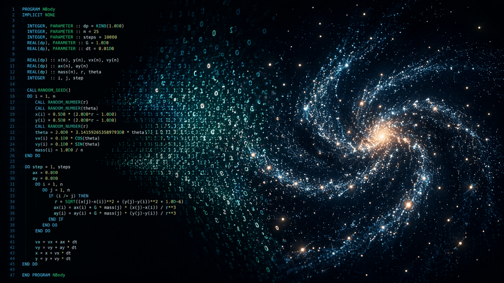
So, I’m going to compile some Fortran code for a simple N-Body simulation, then I’ll try and modernize the output of that code by visualizing the results using Python.

An N-body simulation is a way of asking a computer a very old astronomical question: if you put some objects into space, and let gravity act on all of them at once, what happens next? In this case, “N” is a variable that refers to the number of objects in our sim.

You may have heard the term, “3-body problem” — maybe because of the Netflix series of the same name. In astrophysics, a 2-body problem, say, the Earth and Moon, is fairly routine to deal with mathematically, because one object orbiting another is predictable.

But the 3-body problem refers to the moment when physics stops being neatly solvable, and requires some heavier computation. Motion becomes complex and the three bodies interact with one another.

In our code, we’re going to track the motions of 25 bodies. We’ll spin up a small star cluster, and assign each body a mass, position, and velocity. Then, Fortran will handle the calculations, letting gravity do what gravity does. Every object pulls on every other one, and the computer keeps track of all of it, step by step.

My first step was installing a Fortran compiler on my Linux machine. In this case, we’re using “gfortran” on Fedora Linux. This language has been around since 1957 and its last major update was just in 2023, so it’s fairly modern, despite its early roots in punch-card computing. Not bad for a language nearly 70 years old.

Next, I tweaked the code for the N-Body sim, compiled it, and ran the resulting executable. This only took a fraction of a second. The program produced the CSV output file, containing lines indicating each object name, its mass, it’s position in 2D space, and its direction and velocity.

This is the type of data astronomers used to collect: Text on a page with numbers indicating some sort of change over time. On the surface, this isn’t very useful, because it isn’t visual. We could plot it out on graph paper, but why do that when Python is available?

We can compose a little Python script to draws the star locations frame-by-frame, and output a 6-minute moving visualization of the objects. A programming library called MatPlotLib is doing the heavy lifting here. We’ll bounce out the resulting animation as an MPEG-4 movie for easy viewing.

And there it is, our cluster swirling around hypnotically, stars influencing one another according to Newton’s laws, all being tossed asunder. It kind of looks like a computer simulation from the early 1980s.

If you’d like to tinker with this code yourself, I’ll make all my scripts, and the movie of the simulation, available in the show notes.

After a quick break we’ll be back with this week’s night sky. Stay with us.

Welcome back.

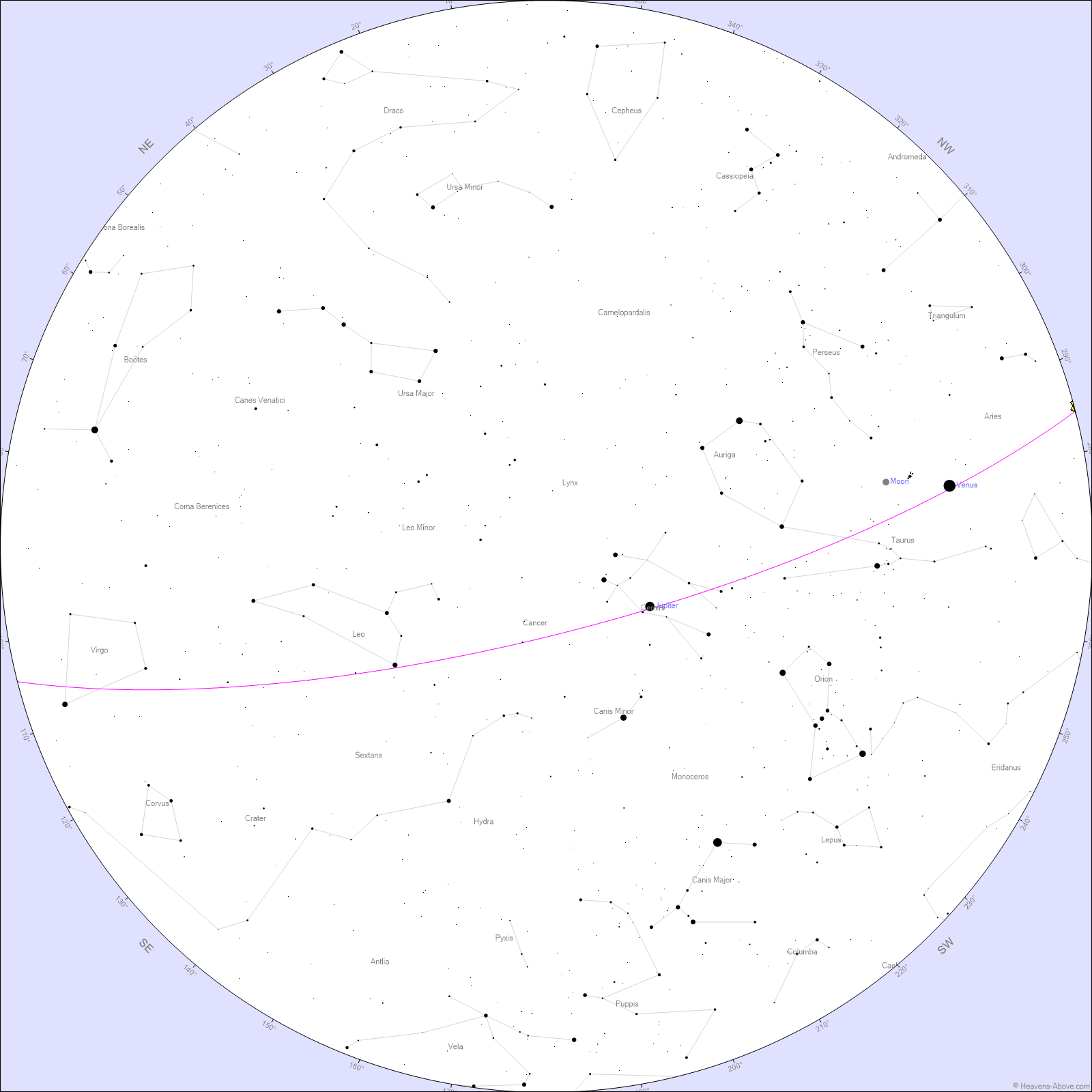
As we step outside this week, the sky greets us in a quiet, reflective mood, still recovering from the darkness of the new moon just a few days prior on April 17. Now, a delicate waxing crescent begins to return to the evening sky.

Look to the western horizon just after sunset. The Moon will be low and subtle. You’ll likely be able to spot Earthshine on the moon’s shadowed side. That’s sunlight reflected off our own planet and back onto the Moon’s surface.

While the Moon quietly returns, something more dynamic is unfolding overhead. The Lyrid meteor shower is active this week, peaking around the night of April 21 into the early hours of April 22.

Under good conditions, you might see 10 to 20 meteors per hour—fast, bright streaks that sometimes leave glowing trails behind. The radiant point lies in the constellation Lyra, near the bright star Vega, but as always, you don’t need to look directly at the radiant. Just get comfortable, look up, and let the sky come to you. With the Moon still in a thin crescent phase, conditions this year are especially favorable.

If you head out just after sunset, one object will immediately grab your attention. That brilliant point of light low in the west is Venus, still dominating the evening sky. On the 19th Venus appears near the young crescent Moon, forming a beautiful pairing in twilight.

Jupiter is still high in the sky, just look almost straight up and search for the brightest point of light.

Mars, Mercury and Saturn are in a very tight grouping, but only visible in the moments just before sunrise, low on the eastern horizon. You’ll likely have a hard time seeing them in the Sun’s glare.

With the Moon still modest in brightness, this is a good week to explore a few deeper targets, especially if you give yourself an hour or two after sunset.

If you’re using binoculars or a small telescope, consider these: Messier 3, a dense, ancient globular cluster rising in the east, and one of the finest of its kind.

Messier 13, The Great Cluster in Hercules, is still climbing higher each night.

And Messier 81 and 82 are a beautiful galaxy pair in Ursa Major, especially under darker skies. And for something a bit more delicate, look for the Ring Nebula, a faint smoke ring suspended in space near Vega.

Vega is in the constellation, Lyra, which is the radiant of the Lyrids meteor shower we just mentioned.

Leo is a prominent constellation of the season, and around April 24, the Moon will pass near it. Look for it’s backward question mark shape, known as the “sickle” anchored by the bright star Regulus.

That’s going to do it for this week. If you found this episode interesting, please share it with a friend who might enjoy it. The easiest way to do that is by sending folks to our website, startrails.show. And if you want to support the show, use the link on the site to buy me a coffee. It really helps!

Be sure to follow Star Trails on Bluesky and YouTube — links are in the show notes. Until we meet again beneath the stars … clear skies everyone!